Conclusions
- Let's try to find a common theme for all three Tables. We can use hyperlinks to go to specific places and come back again. How about going to the level of the electron to see what each Table has to say about it? From Table 1 we find the electron may be a negative value since the Fibonacci ratio +1/2 ends below the level of the electron. From Table 3 we find the energy level....e=Electron = .510998902 Mev/(c^2)..1998 NIST value. This might be meaningful, only to a good mathematician.
- Let's try "Atomic Values": Using these atomic values: p= Proton = 938.271998, n=Neutron = 939.56533, e=Electron = .510998902, [(p+n)*10] + e = 18778.88428 = R. Again, only a good mathematician would know what to do with this information.
- In a new approach, all Fibonacci ratios can be found in both Table 1 and Table 2, sections "Value" and "Term number, k"
- For Example: On the premise that the electron and the human body both represent a quantum unit (Sarfatti or Young?), I searched for the Fibonacci number (55/89) that is in Table 1, section "Body", and which gives a correlation in Table 2. This will occur with every other Fibonacci ratio within the range of both Tables. Fibonacci number 55 now seems to tie the Organs (34/55) and Body (55/89) sections of Table 1, with Table 2 THE AURIC TIME SCALE AND THE MAYAN FACTOR under "Fibonacci Series Term u10" (Col. 1) and "Term v9" (Col. 4), plus the "Value of Phik" (Col. 6) = 76.01 which should imply 76 multiples of Phi ratio from a base position of "Term u1", "Fibonacci 0" or "Term vk = v0. A review of the PDF document is needed for what these terms mean in relation to the Solar-Planetary Synchronism (SPS) Table.
- Here's one that might open your eyes a bit: Keep the previous paragraphs' "76 multiples" of the "Body" ratio 55/89 in mind. 76 shows up multiple times in another solar system study based upon Phi, called "Exponential Order in the Solar System. Spira Solaris Archytas-Mirabilis III". Let's begin searching all the 76's in Spira Solaris, in Reference, below, and if you keep following the link, you'll find yourself right back here. You'll also find that 76 is a Lucas number, which acts like the opposite spiral side to the Phi spiral side, together creating a cadeusus, only the Lucas series is slightly different than the Phi series. Very interesting. Begin here- SOL1-11.
REFERENCES:
1. The Phi Tree (GIF) from GUT MU27 Theory, Phi Physics by Alexander Muvrin
2. THE AURIC TIME SCALE AND THE MAYAN FACTOR (PDF) or Demography, Seismicity And History Of Great Revelations In The Light Of The Solar-Planetary Synchronism by Sergey Smelyakov, Yuri Karpenko.
3. The 26 Levels and Duration of the Temporal Hierarchy x 64 by O.E.Oeric
4. The Quran and the Number 19
5. New Math, New Understanding by D.K.Baily
The unique reinterpretation of gematric 144 may lead to new insight:
The relationship between 36 and 39.37, 36/39.37=0.914401829, the usual case presented here is one of nine places with a zero at midpoint. In rounding, if the number preceding the zero was insufficient to warrant a carry that affected the number on the left side of the zero, it was dropped. Therefore, 0.914401829 becomes 0.9144. This number indicates two main things. Nine being the largest single integer, its use indicates a maximum. The number 144 is indicative
of time squared, as its base of 12 is the base time number. The implications then are 144x2. A form of this number that is found when working this that is considered a square in effect or resultant. 144x2=288, 288^2=82944.
When you look at this as a whole, you will see three applicational paths. These are the reality bases for each of
the three columns mentioned before and should be noted for their respective importance. First you have area in
12^2 and the reality volume expressed as 12^3=1728. In the second you have 144x2=288. This is second magnitude of the origin of 288 found in the ethereal. 288^2=82944 is the mathematical base for the third order of magnitude or the spiritual realm.
To show the relative accuracy of these numbers in application, 39.37x0.9144= 35.999928. How much difference would one millionth of an inch make? In measuring a yard of cloth, would you worry about that amount?
Within the expression of light speed can be found the 3/2 ratio when one converts 186624mi/s to miles per
hour.
186624x60=1197440x60=671846400, square root 671846400=25920, and 82944/ 25920=3.2note
that the decimal is the designated control point, and remember that this deals with an exponential ratio.
PART
III. EXPONENTIAL ORDER IN THE SOLAR SYSTEM
by John N. Harris
A. THE
EXPONENTIAL PLANETARY FRAMEWORK
A-1 THE MERCURY Mt-BASED
EXPONENTIAL PLANETARY FRAMEWORK
Although the exponential function P(x) = Mt phix
(x
= -2 to 16, base Mt = 0.240842658 years )
generates successive mean sidereal and mean synodic
periods from IMO to out beyond Pluto, the
resulting exponential function is (naturally enough) based on the
well-known Phi-Series., i.e.,
Fig 4. The Exponential
Period Function P(x)
= Mtk x
( x = - 2, -1, 0, 1, 2,..,16) and the Phi-Series
A-2 THE PHI-SERIES
EXPONENTIAL PLANETARY FRAMEWORK
In fact the mean sidereal
period of Mercury Mk 0
= Mt that provides the initial starting point for the
exponential
period function is not only comparable to phi -3 =
0.236067978..
years, the entire exponential function differs little from the Phi-Series
for exponents x = -3 through
13, the one-year
period and synodic position of Earth included. Thus there is a second and
even simpler exponential planetary framework available that requires Phi
alone, namely the Phi-Series itself, i.e.,
as shown below in Table 1
for the exponents -3 through 11. At which
point the relationship between the Phi-Series and the Lucas
Series begins
to become apparent. Included here with respect to unity are the
Phi-Series
planetary framework mean values for the periods of revolution, the
intermediate
synodic cycles, the mean heliocentric distances and the mean orbital
velocities.

Table 1. The
Phi-Series Exponential Planetary Framework
A-3 THE
INVERSE-VELOCITY RELATIONSHIPS
Next in line for comparison are the inverse-velocity relationships that
link the four
Terrestrial planets and first three Gas Giants. These three
inverse-velocity
relationships were found in Part II to generate mean velocities with
percentile
errors of 0.02%,0.37% and 0.16% respectively
based
on modern estimates for the associated planets. Investigation of the
Phi-based
exponential functions reveals that all three inverse-velocity
relationships
are not only part of these generated frameworks, they are also an
integral
feature of an uninterrupted sequence that extends throughout each of
them.
Nevertheless an intriguing problem remains. In the case of the MtPhi-based
framework, for example, all inverse-velocity relationships exhibit a
consistant
minor error of 0.975% while for the Phi-Series a
similar
situation prevails with a constant error of 0.355%. The first
set
of errors might be explained by the inital constant Mt
(the
modern estimate for the mean sidereal period of Mercury) but there can
be no such explanation in the case of the Phi-Series proper.
To
correct the discrepancies in the first instance a modified base period
for Mercury that produces a planetary structure with exact
inverse-velocity
relationships is required, in other words, an initial constant that
reduces
all errors to zero. As it so happens this can be determined in a
relatively
straightforward manner (see The
Determination of Mt3). The result is a new, entirely phi-based mean
sidereal period for Mercury (Mt3) of 0.2395640
years, thus producing a third exponential planetary framework with Phi
once again
the underlying constant. Even so there still remains a singular
difference.
In the latter the inverse-velocity relationships that linked the
inferior
and superior planets directly, i.e., the Uranus-Venus/Mercury and the
Mars-Saturn/Jupiter
velocities are both exactly the same. Instead of the Venus/Earth
synodic
velocity presently encountered in the present Solar System, however,
the
Uranus/Saturn and Saturn/Uranus synodic velocities (Syn 13 - Syn 11)
provide
the
mean velocity of Earth, again in a synodic location, as shown below
with the full complement of inverse-velocity relationships generated
from
Mt3 and increasing powers (N) of Phi (i.e.,the
exponential function P(x) = Mt3k
x
for x = -2, -1, 0, 1, 2, ...16) with Mt3
the
new base constant:
| N |
PLANETS |
PERIODS |
DISTANCE |
INVERSES |
VELOCITY |
Vi DIFFS |
DIFFERENCES |
| -2 |
IMO |
0.091505 |
0.2030631 |
0.4506252 |
2.2191392 |
2.2191392 |
Next-Neptune |
| -1 |
Synodic |
0.148059 |
0.2798698 |
0.5290272 |
1.8902620 |
1.8902620 |
Syn 17-Syn 15 |
| 0 |
MERCURY |
0.239564 |
0.3857279 |
0.6210700 |
1.6101245 |
1.6101245 |
Neptune-Uranus |
| 1 |
Synodic |
0.387623 |
0.5316260 |
0.7291269 |
1.3715035 |
1.3715035 |
Syn 15-Syn 13 |
| 2 |
VENUS |
0.627187 |
0.7327086 |
0.8559840 |
1.1682461 |
1.1682461 |
Uranus-Saturn |
| 3 |
Earth/Synodic |
1.014810 |
1.0098489 |
1.0049124 |
0.9951117 |
0.9951117 |
Syn 13-Syn 11 |
| 4 |
MARS |
1.641996 |
1.3918149 |
1.1797520 |
0.8476357 |
0.8476357 |
Saturn-Jupiter |
| 5 |
Synodic |
2.656806 |
1.9182560 |
1.3850112 |
0.7220158 |
0.7220158 |
Syn 11-Syn 9 |
| 6 |
AST.BELT |
4.298802 |
2.6438186 |
1.6259824 |
0.6150128 |
0.6150128 |
Jupiter-Ast.Belt |
| 7 |
Synodic |
6.955608 |
3.6438186 |
1.9088789 |
0.5238677 |
0.5238677 |
Syn 9-Syn 7 |
| 8 |
JUPITER |
11.25441 |
5.0220594 |
2.2409952 |
0.4462303 |
0.4462303 |
Ast.Belt-Mars |
| 9 |
Synodic |
18.21002 |
6.9216070 |
2.6308947 |
0.3800988 |
0.3800988 |
Syn 7-Syn 5 |
| 10 |
SATURN |
29.46443 |
9.5396410 |
3.0886309 |
0.3237680 |
0.3237680 |
Mars-Venus |
| 11 |
Synodic |
47.67445 |
13.147922 |
3.6260064 |
0.2757855 |
0.2757855 |
Syn 5-Syn 3 |
| 12 |
URANUS |
77.13888 |
18.121002 |
4.2568771 |
0.2349140 |
0.2349140 |
Venus-Mercury |
| 13 |
Synodic |
124.8133 |
24.975104 |
4.9975098 |
0.2000997 |
0.2000997 |
Syn 3-Syn 1 |
| 14 |
NEPTUNE |
201.9522 |
34.421707 |
5.8670016 |
0.1704448 |
0.1704448 |
Mercury-IMO |
| 15 |
Synodic |
326.7655 |
47.441400 |
6.8877718 |
0.1451848 |
|
|
| 16 |
NEXT |
528.7177 |
65.385672 |
8.0861408 |
0.1236684 |
|
|
Table 2. The Mt3
Based Exponential Planetary Framework
So far the planetary
framework based on the period Mt3
provides the best overall correlation with the Solar System. Moreover,
the twelve mean periods associated with the initial pair of log-linear
segments include three out of the four gas-giants, in other words, 96
percent of the mass and 92 percent of the angular
momentum
in the Solar System while producing an r-squared
correlation
of better than 0.995 with the Solar System
counterparts.
Once again, however, all three exponential frameworks suggest that the
Asteroid Belt and the locations of Earth and Neptune are anomalous. For
the time being, however, it is sufficient to be aware that by utilizing
the Phi-Series, minor variations in the mean sidereal period of Mercury
and successive multiplications of Phi, it proves
possible
to generate complete planetary frameworks that include the mean
periods,
the mean distances and the mean velocities in frameworks that can all
be
extended inwards towards the Sun and outwards beyond the limits of the
Solar System.
B. THE
PHI-SERIES AND THE SOLAR SYSTEM
B.1 THE EXPONENTIAL CONSTANTS
Up to this point the
representations
of the Solar System have been largely logarithmic, two-dimensional in
form
and generally static in nature, despite discussions concerning periods
of revolution, lap cycles, planetary orbits and velocities. Yet the
complexity
of the Solar System, its endless and varying motions, its waxings and
wanings,
its growth and decay, its anomalies and its regularities all suggest it
is something far beyond a mechanical clock or indeed anything that
simplistic.
But at least from the above analysis there appears to be some
justification
for suggesting that an exponential component exists in the structure of
the Solar System, and moreover, that remnants of it remain in the two
log-linear
zones and the three inverse-velocity relationships discussed earlier.
But where does this leave us? According to the methodology applied
to the mean periods of revolution and the intervening synodic periods,
the suspected log-linearity in the Solar System largely translates into
variants of the Phi-Series such that the mean periods (Sidereal and
Synodic)
increase sequentially by successive powers of Phi while the mean
periods
of the planets increase by Phi squared, i.e., relations 5a and 5b:
Relations 5a and 5b.
The Fundamental Period Constants
Correspondingly,
because of the the third law of planetary
motion and the relationship between the mean periods, mean distances
and
mean velocities, the factor Phi 4/3
or
1.899547627 generates the mean planetary distances while the
square
root of the latter generates the mean distances in general:
Relations 6a and 6b.
The Fundamental Distance Constants
Thus with relation 6b we
obtain a constant increase in mean planetary
distances of 1.88995476295... as opposed to the ad hoc multiples
of 2 that belong to the Titius-Bode relationship. But even so, this
still
leaves an unaccounted "gap" between Mars and Jupiter. For more on this
complex topic see Figure 6 and part F below.
C. THE
PHI-BASED EQUIANGULAR PERIOD SPIRAL
Although the above digressions
and what follows next impinge on matters discussed in Part IV and later
sections, returning to the technical side of the matter there seems
little
doubt that the phi-based exponential planetary frameworks can (and
likely
should) be considered in terms of equiangular period spirals based on
relation
5b expressed in the form:
Relation 9. The
Exponential Period Function and Equiangular Period
Spiral [ from Part IV ]
The resulting spiral (see Part IV) is
predicated on the
equiangular "square" dictated
by relation 5b, i.e., the Phi-squared increase in mean planetary
periods.
Thus for example, Figure 6c incorporates the Phi-Series mean sidereal
and
mean synodic periods from Mercury to Mars:
- Phi -3
= 0.236067978 = MERCURY, mean sidereal period
- Phi -2
= 0.381966011 = Mercury-Venus mean synodic period
- Phi -1 =
0.618033988 = VENUS, mean sidereal period
- Phi 0 =
1.000000000 = Venus-Mars mean synodic period; also
the mean sidereal period of EARTH
- Phi 1 =
1.618033988 = MARS, mean sidereal period
Figure 6c. The
Phi-Series Equiangular Period Spiral from Mercury
to Mars
Delineated on the vertical
axis, the mean planetary periods increase by Phi squared per sidereal
revolution
of 360 degrees while the synodic periods occur at the 180-degree
half-cycle
points. Exactly the same configuration could be given for the
Phi-Series
periods for Jupiter, Saturn and Uranus (or indeed any such segment of
the
Phi-Series) since the periods increase in the same manner, whereas a
uniform
(i.e., log-linear) representation necessarily requires logarithmic data
in addition, as shown in the inset. But there is far more to this
equiangular
spiral, for although the above represents Solar System mean periods,
i.e.,
Time, it turns out that to produce corresponding equiangular
distance
and velocity spirals would be entirely redundant, for both sets of
parameters
are already integral features of period spiral itself. The details are
discussed further in Part IV, but small wonder that Jacob Bernoulli
should
have called the equiangular spiral "Spira Mirabilis" and included it on
his tombstone, or that part of the title is retained here, albeit
shared
with Archytas for reasons that will become apparent in the next few
sections.
On a more recent historical
note, investigation reveals that research concerning the spiral form in
related astronomical contexts includes the work of Lothar Komp in 1996
(see F1. below) and William M. Malisoff in 1929. For the latter's
inclusion
of velocities, distances, periods and the logarithmic spiral see
paragraph
(7) in his 1929 letter to the editor of the Science ("Some
New Laws of the Solar System".)
D.
PHYLLOTAXIS AND THE EXPONENTIAL PLANETARY FRAMEWORKS
Although the present treatment
has concentrated on Time, it now becomes necessary to consider
the
results in terms of the relationship between Phi, the Fibonacci Series
and natural growth. In other words, physical considerations concerning
growth itself, with time, "distance" and speed (i.e., rate of growth)
integral
components. So far the generated exponential planetary frameworks have
largely concerned the mean periods, i.e., time, but as understood from
the outset, this was to obtain more data, new methodology and a more
productive
approach to the structure of the Solar System. Carried though all this,
however, were still the inter-relationships between Time, Distance and
Velocity provided by the velocity expansions to the third law of
planetary
motion and the third law itself. Moreover, as can be seen in Figure 6c,
the obvious complexities of the Phi Series in this specific
astronomical
context reveal that the exact values for the mean periods also
occur
elsewhere in the table among the mean Velocities (e.g., the
mean
sidereal period of Mars and the mean velocity of Mercury; see also
Table
1) in a complex, if not distinctly "ourobotic" context that will be
discussed
in later Sections. As for the occurrence of the Phi Series in the
present
context, those unfamiliar with the subject might wish to bear in mind
that
Phi, the Fibonacci, Lucas and related series, far from being confined
to
plant and animal growth alone, occur in numerous diverse
contexts over an enormous range that extends from the structure of
quasi-crystals
out to the very structure of spiral galaxies. And this being so, should
there really be any great surprise if Phi should also prove to be an
underlying
element in the structure of planetary systems?
It has long been
recognized that although Phi and the Fibonacci Series are intimately
related
to the subject of natural growth that they are hardly limited to these
two fields alone. Remaining with the Phi-Series, Jay Kappraff 3
points out that the French architect Le Corbusier "developed
a linear scale of lengths based on the irrational number (phi), the
golden
mean, through the double geometric and Fibonacci (phi) series" for his
Modular
System. The latter's interest in the topic is explained further in the
following informative passage from Jay Kappraff's CONNECTIONS
: The Geometric Bridge between Art and Science:
As a young man, Le
Coubusier
studied the elaborate spiral patterns of stalks, or paristiches as they
are called, on the surface of pine cones, sunflowers, pineapples, and
other
plants. This led him to make certain observations about plant growth
that
have been known to botanists for over a century.
Plants, such as sunflowers, grow
by laying down leaves or stalks on an approximately planar surface. The
stalks are placed successively around the periphery of the surface.
Other
plants such as pineapples or pinecones lay down their stalks on the
surface
of a distorted cylinder. Each stalk is displaced from the preceding
stalk
by a constant angle as measured from the base of the plant, coupled
with
a radial motion either inward or outward from the center for the case
of
the sunflower [see Figure 3.21 (b)] or up a spiral ramp as on the
surface
of the pineapple. The angular displacement is called the divergence
angle and is related to the golden mean. The radial or vertical
motion
is measured by the pitch h. The dynamics of plant growth
can be described by and h; we will explore this further
in
Section 6.9 [Coxeter, 1953].
Each stalk lies on two
nearly
orthogonally intersecting logarithmic spirals, one clockwise and the
other
counterclockwise. The numbers of counterclockwise and clockwise spirals
on the surface of the plants are generally successive numbers from the
F series, but for some species of plants they are successive numbers
from
other Fibonacci series such as the Lucas series. These successive
numbers
are called the phyllotaxis numbers of the plant.
For example, there are 55 clockwise and 89 counterclockwise
spirals
lying on the surface of the sunflower; thus sunflowers are said to have
55, 89 phyllotaxis. On the other hand, pineapples are examples of 5, 8
phyllotaxis (although, since 13 counterclockwise spirals are also
evident
on the surface of a pineapple, it is sometimes referred to as 5, 8, 13
phyllotaxis). We will analyze the surface structure of the
pineapple
in greater detail in Section 6.9.
3.7.2 Nature responds to
a
physical constraint After more than 100 years of study, just
what
causes plants to grow in accord with the dictates of Fibonacci series
and
the golden mean remains a mystery. However, recent studies suggest some
promising hypotheses as to why such patterns occur [Jean, 1984],
[Marzec
and Kappraff, 1983], [Erickson, 1983].
A model of plant growth developed
by Alan Turing states that the elaborate patterns observed on the
surface
of plants are the consequence of a simple growth principle, namely,
that
new growth occurs in places "where there is the most room," and some
kind
of as-yet undiscovered growth hormone orchestrates this process.
However,
Roger Jean suggests that a phenomenological explanation based on
diffusion
is not necessary to explain phyllotaxis. Rather, the particular
geometry
observed in plants may be the result of minimizing an entropy
functionsuch
as he introduces in his paper [1990].
Actual measurements and
theoretical
considerations indicate that both Turing's diffusion model and Jean's
entropy
model are best satisfied when successive stalks are laid down at
regular
intervals of 2Pi /Phi^ 2 radians, or 137.5 degrees about a growth centerr,
as Figure 3.22 illustrates for a celery plant. The centers of gravity
of
several stalks conform to this principle. One clockwise and one
counterclockwise
logarithmic spiral wind through the stalks giving an example of 1,1
phyllotaxis.
The points representing the
centers
of gravity are projected onto the circumference of a circle in Figure
3.23,
and points corresponding to the sequence of successive iterations of
the
divergence angle, 2Pi n/Phi^ 2, are shown for values of n
from 1 to 10 placed in 10 equal sectors of the circle. Notice how the
corresponding
stalks are placed so that only one stalk occurs in each sector. This is
a consequence of the following spacing theorem that is used by computer
scientists for efficient parsing schemes [Knuth, 1980].
Theorem 3.3 Let x
be any irrational number. When the points [x] f, [2x] f,
[3x] f,..., [nx] f are placed on the
line
segment [0,1], the n + 1 resulting line segments have at most
three
different lengths.
Moreover, [(n + 1)x]
f will
fall into one of the largest existing segments. ( [ ] f means
"fractional part of ").
Here clock arithmetic based on the
unit
interval, or mod 1 as mathematicians refer to it, is used, as shown in
Figure 3.24, in place of the interval mod 2pi around the plant stem. It
turns out that segments of various lengths are created and destroyed in
a first-in-first-out manner. Of course, some irrational numbers are
better
than others at spacing intervals evenly. For example, an irrational
that
is near 0 or I will start out with many small intervals and one large
one.
Marzec and Kappraff [1983] have shown that the two numbers 1/Phi and
1/Phi^2
lead to the "most uniformly distributed" sequence among all numbers
between
Phi and 1. These numbers section the largest interval into the golden
mean
ratio,Phi :l, much as the blue series breaks the intervals of the red
series
in the golden ratio.
Thus nature provides a
system
for proportioning the growth of plants that satisfies the three canons
of architecture (see Section 1.1). All modules (stalks) are isotropic
(identical)
and they are related to the whole structure of the plant through
self-similar
spirals proportioned by the golden mean. As the plant responds to the
unpredictable
elements of wind, rain, etc., enough variation is built into the
patterns
to make the outward appearance aesthetically appealing (non-monotonous).
This may also explain why Le Corbusier was inspired by plant growth to
recreate some of its aspects as part of the Modular system.
(Jay Kappraff, Chapter 3.7.
The Golden Mean and Patterns of Plant Growth, CONNECTIONS
: The Geometric Bridge between Art and Science, McGraw-Hill, Inc.
New
York, 1991:89-96, bold emphases supplied. See also Dr. Ron
Knott's
extensive treatment The
Fibonacci Numbers and the Golden Section, the latter's related
links and the The
Phyllotaxis
Home Page of Smith University)
A great deal of additional
information concerning this complex topic is
obtainable from the above work and the other references, but for the
present
it is sufficient to return to the ongoing line of inquiry, noting from
the various examples cited, that actual phyllotaxic ratios in nature do
not necessarily produce Phi itself--the limiting value of Fibonacci and
Lucas ratios--but numbers obtained from ratios much closer to the
commencing
sequence: 1,1,2,3,5,8,13,21,... For example, the ratios 8:5 = 1.6, 13:8
= 1.625 and somewhat closer to Phi, the ratio 89:55 that results in
1.6181818...
With respect to the Phi-series
and the exponential planetary frameworks under consideration, accepting
(a) that an exponential component does exist in the structure
of
the Solar System, and (b) that the inverse-velocity relationships are
indeed an integral feature of the latter, then it becomes possible to
consider
phyllotaxis in this explicit context, especially since the spiral form
can be considered to be operating here also. At which point it may be
recalled
that in seeking to reduce the common minor deviations in the
inverse-velocity
relationships in the Phi-based planetary frameworks a substitute base
period
for Mercury (Mt3 = 0.2395640) years was
applied
and Phi retained as the constant of linearity. However, although the
determination
of the new base period Mt3 was necessary in terms of the
initial framework, there was nevertheless another way that the common
deviations
could have been reduced to zero, namely the
substitution
of a slightly different value for the major constant Phi itself.
Or, if one wishes, the establishment of a practical ratio similar to
those
discussed above that nevertheless reduced all inverse-velocity errors
to
zero. This requirement is readily achieved by back-solving, resulting
in
the retention of the present day estimate for the mean sidereal period
of Mercury (Mt = 0.240827 years) as the base period but
the
substitution of a a new, slightly lower value of
1.6171413367027
for
the constant of linearity. With this substitution the minor deviations
in the inverse-velocity relationships are still reduced to zero while
the
resulting exponential planetary framework is found to differ only
marginally
from the other three (see Table 3 below).
The question that now arises
is of considerable interest, for how does this new constant of
linearity
compare with the Fibonacci and Lucas ratios discussed above in
association
with natural growth? Although not entirely comparable, it turns out
that
the zeroing constant is indeed close to some of the phyllotaxic ratios
in question, slightly lower, in fact, than the Sunflower's 89:55
phyllotaxis.
SOL1
In other words, the value in question--1.617141336703
--is
closest to the Lucas Series ratio 76
/ 47 followed by the Fibonacci
Series ratio of
55 / 34.
The occurrence of the Lucas ratio in this context is perhaps the least
surprising given the well-known relationship that exists between the
Phi
Series and the Lucas Series, namely that the difference between the two
is the value obtained from reciprocal exponent of the generating power
applied in the former.
SOL2
For example, in the Phi-Series exponential
planetary
framework the theoretical mean sidereal period of Uranus
(76.0131556174..
years) is generated by Phi raised to the ninth power, while Lucas
number
76 is less than this by exactly Phi to the minus ninth power,
i.e.,
0.0131556174.., and the same applies in the case of the eighth powers
and
the 47-year period, and so on.
SOL3
But is it pure coincidence that the
76 and 47-year periods correspond to the respective Phi
Series
periods for Uranus and the Saturn-Uranus synodic? And does the Lucas
Series
predominate here, or is there a Fibonacci component as suggested by
proximity
of the 55:34 ratio? Either way, there is little variance
between
the new exponential periods of the Lucas-Fibonacci (MtLF)
framework
and those provided by Mt3 and the two
previous
frameworks as shown in Table 3, which features the modern estimate for
the mean sidereal period of Mercury for the initial exponential
planetary
framework (Mt-based) and also the last variant that employs the
modified
constant of linearity. Noteworthy in the MtLF-based data (but possibly
coincidental) is the unforced correlation between the value for the
mean
sidereal period of Saturn of 29.45867 years in the latter and the
modern
estimate of 29.45252 years.
Table 3. Comparison
between Solar System Periods and the four exponential
Frameworks.
As explained above, the
MtLF exponential planetary framework also provides error-free
inverse-velocity
relationships, which perhaps suggests that it should provide the
preferred
planetary framework. The following log-linear representation of the
latter
as the diagonal reference line is applied to compress of the range of
the
periods and facilitate the comparison between the exponential
frameworks
and Solar system parameters. Here with the diagonal providing the
reference
frame, deviations above and below the line represent longer and shorter
periods respectively and thus also deviations in heliocentric distance,
i.e., the greater distance above the line the further out for from the
Sun, and below the line, the closer in with respect to the frame of
reference.
Thus the expected deviations for Pluto, Neptune, Mars and to a lesser
extent
Uranus are all evident, as is the suggested location of Earth in the
synodic
position between Venus and Mars. Also included in the comparison is the
Mars-Jupiter Mean and associated synodics on either side. One other
point
of interest is the suggestion of oscillatory "quenching" among the gas
giants (Neptune and Uranus especially) from the outer regions inwards
towards
the lower.
Figure 5. The MtLF
Mean Periods and the Solar System: Mars-Jupiter
Mean included
E. SIMILARITIES AND
DIFFERENCES
A visual
comparison
between the twelve mean periods of the Mt3-based
planetary
framework and Solar System mean data is provided in Figure
5 (for data concerning Neptune and Pluto see Table 3).
The next and outermost theoretical planetary position (period:
526.8669
years; mean distance: 65.233 A.U.) provides the
inverse-velocity
data for IMO although there is no known planet in the
region.
However, it is relevant to note here that Clyde W. Tombaugh (the
discoverer
of Pluto) wrote in 1980 that the search for a tenth Solar System planet
occasioned a number of reports, mostly arising from observed
irregularities
in the orbits of known objects. Although it remained unconfirmed, a
planet
with a mean distance of 65.5 A.U. was in
fact
proposed by Joseph L. Brady of the Lawrence Livermore Laboratory,
University
of California in 1972.4 Since
that time further proposals concerning a possible planet in the outer
regions
have been made by Van Flandern and Harrington, (50 A.U.-100
AU.),5
Whitmire
and Matese (80 A.U.),6
Anderson (78-100 A.U.),7 and
Powell (60.8 A.U., later modified to 39.8 A.U.)8
To
date no tenth planet has been found, but most of these proposals
require
planets with highly inclined orbits, large eccentricities, and
relatively
long intervals between returns, all of which complicate confirmation,
especially
for small objects.
However, further delineation on a wider scale
may eventually be forthcoming from the gravity-based analyses of
Aleksandr
N. Timofeev, Vladimir A. Timofeev and Lubov G. Timofeeva;9
see
also Aleksandr Timofeev's: Two
fundamental laws of nature in the gravity field.
In terms of departures from the norm perhaps the most
difficult anomaly
to accept is that Earth may currently be occupying a resonant synodic
location between Venus and Mars. The establishment of the
heliocentric concept notwithstanding, it would still appear
inordinately
difficult to perceive the position of Earth as anything other than an
immutable
and unquestioned constant. However, the relatively recently advent of
Chaos
Theory, its application in astronomical contexts and the investigations
carried out by Sussman,10
Wisdom,11 Kerr,12
Milani,13 Laskar,14,16, 17
and others have now changed matters irrevocably. The Solar System can
now
no longer be wound backwards or forwards indefinitely like some
well-oiled
and well understood mechanical device, as Ivars Petersen18
recounted in Newton's Clock: Chaos in the Solar system.
Nor
can the positions of any of its various members be considered
sacrosanct,
not even that of Earth.
Whether Earth has always been
in the synodic location between Venus and Mars and in such complex
resonant
relationships is uncertain, but the zone of habitability is generally
defined
by the orbits of the latter pair of planets, and it is an open question
whether life would necessarily have developed at either extremity, or
if
it had, whether it would have necessarily flourished, given the
large-scale
periodic extinctions which appear to have taken place at Earth's more
advantageous
central synodic location. This even suggests that a fortuitous element
may have played a role in the continuance, if not the very development
of life here on Earth, and that while life may still abound in the
universe,
it may not be quite as common-place as previously supposed. Whether
this
has a direct bearing on the negative results obtained over the last
four
decades by the Search for Extra-Terrestrial Intelligence (SETI) is,
however,
another matter altogether. (For an up-to-date analysis of the search
and
an alternative, see Gerry Zeitlin's 1997-1999 essay: OPEN
SETI: Rethinking the SETI Paradigm and the Future of SETI ).
For present
purposes it may be noted that deviations exist between the Solar System
and the exponential planetary frameworks, and that depending on the
degree
of confidence assigned to the latter, it may be feasible to quantify
these
anomalies in terms of planetary masses, mean distances, and the
conservation
of angular momentum, etc. This still leaves the anomalous position of
Neptune,
but it is possible to suggest a number of scenarios based on
mass-distance
changes that might include a further belt of asteroids and/or cometary
material at approximately 65 astronomical units from the sun
periodically
perturbed by an object or objects in a eccentric polar orbit, etc.
Apart
from the exponential framework itself, very little of this is actually
new, though scenarios based on total angular momentum might well remain
problematic owing to uncertainties concerning the complete inventory
and
total mass of the Solar System itself. On the other hand, new avenues
and new insights concerning the structure of the Solar System have
already
begun to surface; e.g., the Fibonacci-related paper by Aleksandr N
Timofeev
entitled: "Sprouts of New Gravitation Without Mathematical Chimeras of
XX Century."
RE-ASSESSMENT FOR THE
NEW MILLENNIUM
In
looking
back
over the three years that have elapsed since this third section of
Spira
Solaris was first uploaded in 1997 I have come to realize that I have
been
somewhat slow to react and even slower to change in spite of a number
of
positive inputs concerning the present subject that arrived one way or
another via the Internet. This was partly because of an increasing
interest
in the historical side of the matter but also my own inability to
absorb
and act on the various inputs received.
A little
over
a year ago (mid-December 1999) I received an E-Mail and later a written
follow-up concerning a series of Phi-associated planetary relationships
arrived at by Mr. John Shanahan
of Berlin, Germany. The latter provided a modern source for the mean
planetary
data applied in his relationships, but was concerned in part that the
results
for some varied according to differences in modern parameters. In
particular,
based on mean dista
nces of 1.523691 A.U.,
0.387099 A.U. and 9.575616
A.U.
for Mars, Mercury and Saturn respectively, although he arrived at a
close
approximation for Phi via the following route:
his concern was
indeed justified, for only minor differences
in the associated mean distances produced departures from the excellent
value for Phi shown in relation [S1]. But be that as it may, on
examination
it turns out that the relationship is nevertheless directly applicable
to the Phi-Series planetary framework, and moreover, it not only
applies
to the mean distances, but also the mean periods throughout. Actually,
it does lead to Phi when the Phi-Series Mean Periods are
applied, and also the corresponding value for the distances
(1.378240772
) when the distances are applied in turn. The reason for this becomes
clear
when one reduces the periods involved to their associated exponents
although
it is unnecessary to repeat the analysis here. The initial derivation
by
Mr. Shanahan was therefore in one way erroneous, but in another, it
might
well have resulted in an awareness of the Phi-Series planetary
framework.
But this was not the end of the matter anyway, for the latter had
forged
ahead and produced further exponential relationships, including the
following
involving the mean distances of Mercury, Mars, Jupiter and Neptune (the
mean distances used were 0.387099, 1.523691, 5.204829, 30.068963 A.U.
respectively.
The agreement
here is again excellent based on modern
values for the mean distances, but the reader will recall that Jupiter,
Mars and Neptune all deviate from the exponential planetary framework,
the latter especially. Thus one would hardly expect the exponential
equivalent
of this relationship to show any real correlation. But surprisingly, it
does, in fact it produces perfect agreement using the the Phi-Series
mean
distances. But how can this be, with so much divergence between the
mean
distances of the latter framework and the modern estimates? In the case
of Neptune, for example the Phi-Series equivalent is 34.0859 A.U.
compared
to the modern mean distance used above of 30.0689 A.U. and there is
also
a marked difference between the distances for Mars in addition. Then
there
is the difference for Jupiter with a mean distance of 5.203336 A.U.
compared
to the Phi-Series value of 4.97308025 A.U., and also Uranus at
19.191264
A.U. versus 17.9442719 A.U. A puzzle certainly, but also an
opportunity,
for the differences could be considered in terms of adjustments made
with
respect to the exponential planetary framework. Why should there be
adjustments
of this kind in the Solar System? The most likely cause, if not the
most
obvious, would be some change or other in planetary masses and/or
positions.
If so, there are certainly places in the Solar System that immediately
come to mind where this might have taken place--not only the Asteriod
Belt,
but also perhaps, in the region occupied by slightly anomalous Uranus.
Or should one say highly anomalous Uranus with its axis tilted
almost
ninety degrees off the "vertical"--a planet that is truly rolling along
its orbit; or barreling around it, if one wishes. Just how Uranus came
to be in this unusual situation has not been established, although
there
have been a number of theories proposed, as Eric Burgess explains
below,
adding a few more points of interest for good measure:15
The axis
of Uranus is tilted so as to lie almost in the
plane
of its orbit ... one speculation is that there was a catastrophic
collision
with another planetary body early in the planet's history. . . What
could
have caused this axial tilt? One possibility is soon after the planet's
formation it was hit by an Earth-sized body. An impacting speed of
about
64,000 kph might be sufficient, according to some calculations, to push
the planet on its side.. . A major mystery about Uranus is the low heat
flux from the interior ... .all the small (Uranian) satellites have . .
. . extremely dark surfaces. . . .What is this surface material? All
the
Uranian satellites are darker than the satellites of Saturn .. Also the
colour of the surfaces is grey, whereas many other Solar System
satellites
have a tendency towards redness. (Eric Burgess, Uranus and Neptune,
Columbia University Press, New York, 1988:51)
An impacting speed of about
64,000 kph translates into some 17.778 k/sec--an
orbital velocity that corresponds to a distance of 2.7992 A.U., which
places
it in the central region of the Asteriod Belt, another enigma and a
complex
one at that. Again there are various theories that might be considered
with respect to the latter, including either the breakup of a planetary
body in the region and/or the ejection of a sizable amount mass from
it.
So perhaps there are two areas that may have required
adjustment--the
first being a loss of mass within the Asteriod Belt itself, and the
second
involving a possible loss of mass from Uranus, with the event in the
latter
region perhaps responsible for it. In other words, the collision may
not
only have knocked Uranus on its side, it may also have been of such
force
that it chipped off perhaps sufficient mass to require adjustments into
the bargain. Either way the loss of mass would necessarily influence
the
total angular momentum and compensation would be required to maintain
the
conservation of energy. And since orbital angular momentum is a
function
of velocity, mass and distance, the slack would have to be taken up by
an outward movement of one more of the other planets or Uranus itself.
Apart from their
theoretical
nature, there are unfortunately far too many variables in such
scenarios,
yet we do know the masses of the planets, we do have the parameters of
the present Solar System and also the mean values from the exponential
planetary frameworks. As a consequence the total angular momentum can
at
least be calculated in both cases and the difference between the two
examined.
Now at this juncture it is necessary to recognize that it is most
difficult
to obtain any guidance regarding what may or may not have happened to
the
Solar System in the past, even with the frame of reference provided by
the exponential planetary framework. Nevertheless, Relation [S1] does
provide
an initial avenue to explore. But if comparisons with the Solar System
are required, then it would perhaps be better to employ the MtLF-based
planetary framework in so much as it not only retains the modern
sidereal
period for Mercury for its base period, it also gives the closest
correlation
with Saturn, i.e., a mean distance of 9.53842 A.U. compared to the
modern
value of 9.53707 A.U. This means for the same mass there is only a
slight
difference in angular momentum for this planet, whereas the difference
between the Solar System and the exponential framework are considerable
for both Jupiter and Neptune and to a lesser extent, also Uranus.
In seeking the simplest of
initial tests it is possible to immediately focus attention on Uranus,
not only because of the possibility of a catastrophic event, but also
because
relation of [2S], which suggests that both Jupiter and Neptune may have
been two of the planets that underwent adjustments. A further
simplification
is to consider that the event (or events) took place before the
formation of the four terrestrial planets and Pluto. This leaves us the
four major superior planets, and with Saturn virtually unchanged, just
the two adjusting planets (Jupiter and Neptune) plus Uranus, the
possible
prime casualty. All that remains is the Asteriod Belt, and that too may
not have formed to any great extent at this hypothetical stage. Various
scenarios can be suggested, but it still most difficult to assess what
changes may have resulted, or which planet may or may not have played a
role in the readjustment. But there is one thing that can be done above
all else, and that is compare the total angular momentum for the known
planetary masses applied to both sets of planetary distances.
For a total of 446.83728
Earth
masses the angular momentum for the nine Solar System planets relative
to unity is 1179.2179; for the same total mass and the last mentioned
exponential
planetary framework the angular momentum is in turn 1171.4148, thus
smaller
by 7.807458. The breakdown of the Solar System surplus is: +12.52712
for
Jupiter, +1.830719 for Uranus, a mere -0.02073 for Saturn and -6.52966
for Neptune. These discrepancies are the result of the differences in
the
mean distances, i.e, the suspected adjustments, but if so, then what
caused
them? Still focusing on Uranus, we know from the comparison with the
exponential
framework that this planet may have moved further out, possibly an
adjustment
of its own. In other words, to perhaps maintain angular momentum after
losing a certain percentage of its mass, which would not be entirely
surprising
if it had indeed been hit by a sizable chuck streaking out of the inner
solar system faster than a high-velocity bullet. But even so, what then
of the other "adjustees"? Thus the problem expands, and with it the
number
of variables. But there remains one further possibility that can at
least
be checked. If, as suggested earlier, the event in question took place
before
the formation of the four terrestrial planets, then where did their
respective
masses come from? From the collision with Uranus, perhaps, and this too
can be investigated, merely by assigning the total Solar System mass to
the four superior planets in the exponential planetary framework and
finding
what change in mass for Uranus brings the surplus in the angular
momentum
back in line. Recomputed in this manner, the mass of the four
terrestrial
planets and Pluto (1.980278) increases the present mass of Uranus from
14.559 to 16.5393, and somewhat surprisingly, balance is achieved at
16.8348.with
only a further increase in mass of 0.29554.
All of which leaves far too many gaps and other possibilities; but
thanks to Mr Shanahan, it at least serves to emphasize that the
exponential
planetary frameworks discussed here may have some additional validity,
if not additional uses. For more on Mr. Shanahan's
continuing research see the latter's Web
Site.
F.
LUCAS AND FIBONACCI RESONANCES IN THE SOLAR SYSTEM
F.1 LOTHAR KOMP
Up to the present point
the
discussion has concentrated on the baseline provided by mean periods of
revolution (sidereal and synodic), mean heliocentric distances and mean
orbital velocities. In the Solar System itself, however, matters are
far
more complicated owing to the elliptical natures of the planetary
orbits
and differences (although slight) in the inclination of the orbital
planes.
Added to these complications are the various resonances that occur
between
the planets themselves, both real-time and mean motion resonances. As
it
turns out, many of the planetary resonances in the Solar System are
either
Fibonacci or Lucas Series related--resonances that not only incorporate
the ratios 1:2, 2:3, 3:5, 5:8, 8:13 and higher, but also
triples
and in some case quadruple resonances.
It cannot be said that such
occurrences have gone unnoticed, nor can it be said that the
relationship
between the Fibonacci Series and related resonances have not been
equated
with the structure of the Solar Sy
stem in the past. But even with
such
qualifiers it is difficult to understand how recent research on the
subject
carried out by Lothar Komp20 during
the
last decade has languished basically unheralded and unappreciated.
First
published in 1996 in the German-language magazine Fusion and
the
English-language magazine 21st Century the following year
(1997)
in an article entitled: "The Keplerian Harmony of the Planets and Their
Moons," Lothar Komp's work was far more Science than History though
both
subjects were interwoven in a dense, highly informative and original
discourse.
But more to the present point, Lothar Komp's researches dealt in
considerable
detail with the Fibonacci Series in specific astronomical contexts and
spiral forms that included the following:
Systems of
Planets and Moons as "Barred Spirals."
Spiral Galaxies, Logarithmic Spirals and Ratios
A precise hyperbolic cosine distance formula, i.e.,
A Barred Spiral and the
Moons of Neptune
A Barred Spiral and the Moons of Uranus
A Barred Spiral and the Moons Jupiter
A Barred Spiral and the Moons of Saturn
A Barred Spiral and the Outer Planets
A Barred Spiral and the Inner Planets
Synodic and Sidereal motion
Planetary and lunar resonances
Resonances that included rotation rates
Resonances among the Asteroids
Solar Activity and Planetary motion
all inter-spaced with
informative historical asides and due recognition
of the related works of Johannes Kepler, as will be noted later.
In the meantime in view of Lothar Komp's extensive treatment of the
topic it is necessary to accord the precedence of the latter's work
published
in 1996 in addition to the 1929 conclusions of William M. Malisoff
already
noted in section C.
F.2 MEAN MOTION
RESONANCES
Without going into too much
detail, in addition to Lothar Komp's treatment of the 1:2, 2:3,
3:5,
5:8, 8:13 resonances there also exist other perhaps lesser-known
mean
motion resonances, e.g., an interval of 34 years for Earth and Mars
that
corresponds to 18 sidereal revolutions for the latter, while further
complexities
concerning Venus arise when various multiples of 8 years are
investigated,
e.g., the 64-year period with 104 sidereal periods of Venus, 64
sidereal
revolutions of Earth, 40 Venus-Earth synodics and additionally 34
sidereal
revolutions of Mars. Remaining with the latter but using attested
Babylonian
period relations, in 47 years there will be almost 25 sidereal
revolutions
and
SOL4
22 Earth-Mars synodic periods, to which may also be added that in
76
years there are 34 Mars-Jupiter synodic cycles. The Babylonians
possessed
far more period relationships than the few given here; including a
related
79-year period for Mars, 29 and 59-year periods for Saturn, and 12,
71,83,
95, 166, 261 and 427 years for Jupiter (for further details concerning
these periods and their application see Babylonian
Planetary Theory and the Heliocentric concept) in
each instance,
SOL5
while some of the
above periods--especially those of 34, 47 and 76
years are also reflected--perhaps coincidentally--in the two ratios of
primary interest--the Lucas 76:47 and Fibonacci 55:34
ratios.
Then there are the further complexities associated with resonances
in the Asteriod Belt, including the 1:1 mean motion
resonances
of Jupiter-associated asteroids, known mean-motion 3:1, 5:2, 7:3,
2:1 resonance gaps and 3:2, 4:3, 1:1
concentrations.
Such resonances within the Asteroid Belt may also be considered with
respect
to the mean sidereal periods of 1.880751 years and 11.868991
years of Mars and Jupiter respectively and the resulting geometric mean
(MJM) between the two of 4.724682 years
which
is comparable to known 5:2 mean motion resonances. Secondly,
the
Mars-MJM synodic period stands in the ratio of 5:3
with respect to Mars, while the MJM-Jupiter synodic
stands
in a 3:2 ratio with respect to Jupiter, and a number of
further
5:3:2
resonances also occur. Although obvious, it
may be overlooked at times that all integer period relations expressed
in years necessarily include the sidereal revolution of Earth and
hence the
resonances of Earth itself
Figure 6. Log-linear
representation of the Asteriod Belt with Mars-Jupiter
Synodic and MJM (Mean)
Further out among the
anomalous planets Neptune and Pluto there are
additional resonances, and with respect to the former
it
is also known that both Earth and Neptune are locked in similar
resonant
relationships. Denoting synodic periods by Ts, inner and
outer mean sidereal periods by T1 and T2
and
resonant relationships by: T1 : Ts : T2, both planets
are
in fact in 2:1:1 resonant relationships with adjacent
bodies
(Earth with Mars; Neptune with Uranus) while Neptune is also locked in
a further 3:2:1 resonant relationship with Pluto. The
latter's
mean period produces poor results throughout as a base parameter for
the
exponential frameworks, but in comparison to its neighbors the gas
giants,
this small planet is already anomalous on a number of counts.
Undoubtedly
problems exist with the location of Pluto in the present context, but
it
is nevertheless still Neptune that represents the major discrepancy in
the outer regions of the Solar System. Whether resonances among
the four major superior planets will shed any light on the matter
remains
to be seen, but there is far more to this whole matter than mean motion
resonances in any case, since real-time resonances in the Solar System
must also be addressed. The question that now arises is how best to
investigate
these resonances on one hand and display them effectively on the other.
F.3. REAL-TIME
RESONANCES: THE INFERIOR PLANETS
For this purpose the methodology
of Bretagnon and Simon21
adapted
to time-series analysis is particularly useful, especially the power
series
data and formulas for deriving heliocentric distances. The adaptation
(given
in Times Series
Analysis)
will be explained in more detail later but for present purposes it is
sufficient
to note that for any part of a planet's orbit at any point in time the
instantaneous value of the radius vector can be treated as the mean
value
of an equivalent mean distance orbit and consequently also provide
corresponding
periods and velocities for the same. In other words, each planetary
orbit
may be considered in terms of successive mean motion orbits extending
outwards
from the shortest distance at perihelion to the longest at aphelion. In
this way not only the varying distances, but also the velocities and
periods
may be treated as continuous functions over successive intervals.
Instantaneous
values of successive radius vectors may then be used to generate
corresponding
periods that serve to illustrate some of the better-known resonances
among
the inferior and superior planets. With respect to the former,
particularly
the adjacent planets Venus, Earth and Mars there seems little doubt
that
from a dynamic viewpoint Earth's location between Venus and Mars is
highly
complex. In addition to the resonances listed by Lothar Komp it may be
noted that although the Venus-Mars mean synodic period is 0.914224
years, in practice the elliptical nature of the orbits of the three
planets
cause the instantaneous sidereal and synodic velocities to vary widely
and also periodically coincide. But Earth is not only locked in a 2:1:1
resonance with Mars, but also in a 13:5:8 resonant relationship
with Venus, which is itself linked to Mars by a further 3:2:1
resonance.
Moreover, a plot of the true varying sidereal and synodic motion in the
form of time-series data reveals the existence of even more complex
resonant
relationships as seen in see Figure 7 below:
Figure 7. The
Venus-Earth-Mars Resonances and the Lucas Series Numbers
This actual example
computed a number of years ago remains part of a
relatively inconclusive but not entirely negative investigation of
planetary
resonances and their possible inter-relationship with solar activity.
At
that time even the more obvious feature--that all the numbers involved
belong to the Lucas Series, i.e., 1,3,4,7,11 was not noted; nor
were the other resonances encountered examined in terms of the
Fibonacci
Series per se. The present example (which repeats after almost
thirty-two
years) is however but one of a number of approaches that can be applied
to the problem. It may be further noted here that in addition to
occupying
a resonant intermediate synodic location between Venus and Mars, that
the
corresponding inverse-velocity function for Earth may also defined in
terms
of the inverse-velocities of the three adjacent gas giants (the
Uranus-Saturn
and the Saturn-Jupiter synodics respectively) which are in turn subject
to real-time periodic variations of their own.
SOL6
But there still remains the unexplained occurrence of the Lucas 76:47
and Fibonacci 55:34 ratios and why the former gives the better
correction
for the inverse-velocity functions in question. On the other hand,
there
is the apparent linkage between the major superior and the terrestrial
planets provided by the inverse-velocity functions and the undoubted
Fibonacci
relationships that exist among the more massive group of planets,
Jupiter
and Saturn especially.
F.4. REAL-TIME
RESONANCES: THE MAJOR SUPERIOR PLANETS
Perhaps the best known resonance
in the Solar System involves the relative motion of Jupiter with
respect
to Saturn. But before examining this example in detail it is
necessarily
to emphasize the predominance of this pair of planets above all others,
including the adjacent major superior planets Uranus and Neptune. Alone
Jupiter accounts for 71% of the planetary mass in the Solar System and
more than half of the total angular momentum. Saturn comes next with
21%
of the mass and and 25% of the angular momentum; taken together Jupiter
and Saturn thus account for 92% of the mass and more than 85% of the
angular
momentum. The further inclusion of Uranus lifts the totals to 95% and
92%
respectively, while all four major superior planets account for more
than
99% of the planetary mass and more than 99% of the total angular
momentum
in the entire Solar System.
Of the four major planets,
the heliocentric positions of the first three not only compare to
successive
positions on the exponential planetary frameworks, they also permit the
generation of the three inverse-velocity relationships discussed in
Part
II. But there are other considerations to be factored into this complex
equation, for Jupiter is not only the largest planet by far in terms of
size and mass, it is also the swiftest moving major planet, followed in
due order by Saturn (the next most massive) and then Uranus. Neptune at
present represents an anomaly though it obviously cannot be ignored.
But
if one is going to concentrate on the major planets then it would be
logical
to expect that the influence of Jupiter and Saturn would predominate,
followed
next by Uranus. In other words, the three adjacent planets that belong
to the five successive sidereal and synodic periods from Jupiter out to
Uranus from the original log-linear segment. But since the sidereal and
synodic relationships between Jupiter, Saturn and Uranus have long been
known and to some extent researched, whatever it is that remains to be
determined must be more than this alone, or even perhaps entirely
different.
Then again, perhaps it is something relatively simple but difficult to
check exhaustively. Now at least the exponential planetary frameworks
provide
bases for comparison, as do the inverse-velocity relationships.
Finally,
the phyllotaxic Fibonacci/Lucas ratios at least permit the narrowing of
the inquiry to an investigation of real-time resonances among the the
four
most massive objects in the Solar System.
F.5. THE JUPITER-SATURN
CYCLES AND URANUS
As mentioned earlier, the
present methods were first adapted a decade or more ago to generate
real-time
data to investigate the possible influence of planetary motion on Solar
Activity cycles--an investigation that included resonances, but not
exhaustively.
Here the same methods can be directed towards more specific goals,
though
it is as well to be aware of the complexities in attempting to come to
terms with interactions that involve multiple elliptical orbits and
varying
motion. A real-time period function for Jupiter will vary on either
side
of the mean sidereal period by the range permitted by the planet's
eccentricity,
in this case approximately 11 to 12.75 years and a similar situation
prevails
in the case of Saturn with a range of approximately 27 to 32 years. The
more complex Jupiter-Saturn synodic cycle on the other hand
has
a somewhat wider theoretical range (approximately 17 to 24 years) with
corresponding data derived from the synodic formula and periods
obtained
from the Jupiter-Saturn radius vectors. Time-series results in this
case
provide sinusoidal period functions that follow the variations of the
respective
radius vectors over time. Thus over approximately 59 years the 5:3:2
resonances of Jupiter and Saturn will be displayed as five sinusoidal
waveforms
for the former (i.e., 5 sidereal cycles), two sinusoidal cycles for
Saturn,
plus a three-cycle synodic waveform that maps the relative but varying
motion of Jupiter with respect to Saturn over the same interval.
"Resonances"
occur when all three waveforms coincide--three times in the present
example.
But before proceeding there are two further matters that require
explanation
and emphasis. The first is that as long as the basic 5:3:2 relationship
for Jupiter and Saturn holds, multiplications need not stop at the
approximate
59 year period; nor for that matter, need the well-known 1:1:2
resonance
of Uranus with respect to Neptune necessarily remain with unity (the
latter
provided by the mean period of Neptune), i.e.,
Figure 8.
Jupiter-Saturn and Uranus-Neptune Resonances and the Fibonacci
Series, 1940-1990.
More to the present point,
to investigate possible interactions between
the 5:3:2 Jupiter-Saturn resonance at about 59 years and
the 2:1:1 Uranus-Neptune resonance, the real time functions for
the former pair can be amplified, but not by merely tripling the 59
years.
Rather, as in the case below that concerns the relationship between the
two major planets, the Jupiter-Saturn values can be raised by the
Fibonacci
triple 13:8:5 to bring them into the operating range of the
Uranus
Neptune cycle. This is not at all intuitive, for the average value for
the
periods obtained from this mean-value multiplication appear to be too
low,
i.e., their average is about 153.5 years compared to the 165-year mean
period of Neptune and the mean synodic period of Uranus of 171 years.
But
these are mean values that in effect mask the real variance that occurs
with multiple elliptical orbits. Moreover, the following time series
plot
of the 13:8:5 Jupiter-Saturn
real-time data over one Uranus-Neptune
synodic cycle from 1890 to 1990 (7300 simultaneous data points
generated
in 5-day intervals for each waveform) reveals illuminating and
unexpected
crossover points as the vertical axis shifts upward, including the
intersection
of the Uranus-Neptune synodic waveform with the Jupiter-Saturn cycle:
Figure 8b. Multiple
Jupiter-Saturn and Uranus-Neptune Resonances,
1890-1990.
At this juncture the
matter begins to focus more firmly on the Fibonacci
and Lucas Series, for in seeking to embrace the latter it seems that
while
it is still necessary to concentrate on the relative motion of Jupiter
with respect to Saturn, the relative motion of Jupiter with respect
to Uranus also has a significant role to play. The
mean
value of this period is readily obtained from the the mean sidereal
periods
of Jupiter and Uranus by way of the general synodic formula. Given to
the
sixth decimal the mean synodic period of Jupiter with respect to
Uranus
thus turns out to be 13.820371 years. What follows next is perhaps
surprising,
for in dealing with multiple harmonics--which is essentially what is
under
consideration here--it is one thing to invoke Fibonacci variants of the
basic 5:3:2 resonant relationship between Jupiter and Saturn, and quite
another to expect that the Jupiter-Uranus harmonics would relate to the
Lucas Series in this precise context, especially in an opposite sense.
Nor for that matter is it likely that one would anticipate that while
it
is necessary to reverse the order of the fibonacci triples to maintain
the resonant relationship between Jupiter and Saturn (i.e., 5:3:2 to
obtain
5 cycles of Jupiter, 3 Synodics and 2 cycles of Saturn in approximately
59 years, and so on), that the Lucas harmonic expansion would follow
its
normal order, i.e., 4, 7, 11, 18, 29, ... etc. But this being said, we
are at least familiar with the Phi-Series planetary frameworks, the
relationship
between the latter and the Lucas Series and we are already dealing with
the mean periods of revolution and synodic cycles expressed in years in
both contexts. Again, however, bearing in mind the variance that
results
from the true orbital motions of the three planets in question, the
relationship
between the reversed Fibonacci triples and the Lucas harmonics is still
not immediately apparent. One of the main reasons for this is that it
only
becomes clear after the multiple periods of the Jupiter-Saturn triples
are averaged, and then only with the longer intervals is the
relationship
easily detectable. For example, based on a mean sidereal period of
11.869237
years for Jupiter, a corresponding mean synodic period 19.881324 years
and mean sidereal period for Saturn of 29.452520 years, the fifth,
third
and second multiples (i.e., the 5:3:2 resonance) occur after 59.346
years,
59.644 years and 58.905 years respectively, whereas the average for all
three products is 59.298 years. The fourth (4) Lucas augmentation of
the
Jupiter-Uranus mean synodic period on the other hand occurs after
55.282
years--a loose correlation easily dismissed as a chance occurrence.
However,
further investigation reveals that the 5:3:2 Jupiter-Saturn and
Jupiter-Uranus
Lucas multiple 4 are seemingly co-associated, for the next Lucas number
(7) is similarly associated with the next reversed Fibonacci
triple
after 5:3:2, and as the two sets both proceed to their larger numbers,
the difference between the averages of the Fibonacci triples and the
Lucas
multipliers becomes increasingly less.
SOL7
Thus by the time the 89:55:34
Fibonacci
triple is reached the average of 1050.41 years is more closely
approximated
by the 1050.38 years obtained from the 76th multiple of the mean
Jupiter-Uranus
synodic cycle. In other words, the Fibonacci and Lucas assignments
proceed
sequentially, side-by-side in strict order. Thus the harmonic Fibonacci
triples of the Jupiter-Saturn triad are related to the Lucas harmonics
of the Jupiter-Uranus synodic cycle in the following manner for the
given
periods (rounded here to the nearest year for clarity and convenience):
5
3 -Lucas 4 ( 59 Years )
2
8
5
Lucas 7 ( 94 Years )
3
13
8 -Lucas 11 ( 153 Years )
5
21
13
Lucas 18 ( 248 Years )
8
34
21 -Lucas 29 ( 401 Years )
13
55
34 -Lucas 47 ( 649 Years )
21
SOL8
89
55 -Lucas 76 ( 1050 Years )
34
As a consequence of the above, the ratios of the successive averages
(F Means) move towards the limiting value Phi as the periods increase,
until between the time of the Fibonacci triple 55:34:21 / Lucas
product 47, and Fibonacci 89:55:34 / Lucas product 76
the approximations: 1.617413 and 1.618271 are obtained, values close to
that of the zeroing constant of linearity of 1.617141 applied
in the MtLF exponential planetary framework.The manner in which the two
sequences proceed towards the limiting value is shown below in Table 4
and Figure 9. The latter also includes the twin-serpent caduceus since
these two intertwining sequences -- from the present viewpoint at least
provide the mathematical
and
astronomical underpinnings for this most ancient and complex symbol,
historical
complexities notwithstanding. Firstly the single intertwining ratios of
the Fibonacci Series about the mean, later followed by the Pythagorean
union of female and male (in the Egyptian sense "Upper" and "Lower") of
the Fibonacci: 1, 2, 3, 5,.. and Lucas: 1, 3,
4, 7,.. series respectively.
Figure 9. The
convergence towards the limit Phi by the Fibonacci
and Lucas Series Ratios.
Or is there more to
this matter in any case, including wider horizons with additional
degrees of complexity?
Consider, for example, the detailed arguments presented in the
following:
Table 4. The
Jupiter-Saturn, Jupiter-Uranus Resonances and the Fibonacci/Lucas
Series
SOL9
Returning to the matter at
hand, however, we have now arrive at the 76:47
Lucas ratio in true consort with
the 55:34 Fibonacci ratio, with Lucas harmonics always
occupying
the position between the highest and next highest values in the
associated
Fibonacci triple.
SOL10
And here, as can be seen in Figure 10 --
real-time 89:55:34 multiples of the Jupiter-Saturn cycles and
the
76th Jupiter-Uranus cycle
the latter component also moves towards
the nexus of the Jupiter-Saturn cycles, and this increasingly so with
time.
At which point it seems both relevant and useful to redirect the reader
to Kurt Papke's Animation
of Binet's Formula available on the Internet since 1998--a
presentation
that (speaking for myself, at least) only now comes into clearer focus.
SOL11
Figure 10. The 89:55:34
Jupiter-Saturn and 76 Jupiter-Uranus Cycles,
1940-2000.
As a first approximation
it therefore seems that the relative motions
of Jupiter, Saturn and Uranus, and predominantly that of the first--the
largest, swiftest and most massive of the three are intimately
associated
with the Golden Ratio. Not included here, yet likely also involved are
the relative motions of Saturn with respect to Uranus, the motion of
Saturn
with respect to Neptune, and additional complications arising out the
dominance
provided by Jupiter with respect to all three. Nevertheless, the
situation
may be summarized at this initial stage in terms of the relative
motions
of the three major superior planets Jupiter, Saturn and Uranus as
follows:
Figure 11. The
Fundamental Fibonacci and Lucas Resonances; Jupiter-Saturn,
Jupiter-Uranus
Where does this leave us? Is
it that surprising that the relative motion of Jupiter--firstly with
respect
to Saturn, and secondly with respect to Uranus--should predominate in
the
Solar System? And also, that the Golden Ratio should underlay so much
order
and proportion in addition? Where does it all originate? That question
no doubt belongs to philosophical debates concerning the first of
things,
but if it is the product of the rel
ative motions of Jupiter, Saturn
and
Uranus, then it is little wonder that such ordering occurs if it is
indeed
resonating throughout the Solar System.
The above somewhat limited
discussion necessarily concerns complex waveforms and motions for the
mean, varying
and extremal values dictated by elliptical orbits.
Although one could suggest that both the Fibonacci and the Lucas Series
are embedded in the Solar System, it might be more accurate to say that
they are in fact pulsating through it, and perhaps have been since time
immemorial.
GOLDEN
DIGRESSIONS
1. Babylonian.
2. Egyptian
REFERENCES
- West, John Anthony, Serpent
in the Sky:
The High Wisdom of Ancient Egypt, Quest Books, Wheaton,1993.
- Gillings, Richard J.
Mathematics in the Time
of the Pharohs, Dover Books, New York, 1982.
- Kappraff, Jay. CONNECTIONS
: The Geometric
Bridge between Art and Science, McGraw-Hill, Inc. New York, 1991.
- Brady, J., cited in Out
of the Darkness: the Planet Pluto,
by Clyde Tombaugh and Patrick Moore, Stackpole Books, Harrisburg, Pa.,
1980:201.
- Littman, M. Planets
Beyond, John Wiley and Sons, New York,
1988:198.
- Op.cit., p.202.
- Op.cit., p.204.
- Op.cit,
pp.205-206.
- Aleksandr N. Timofeev,
Vladimir A. Timofeev, Lubov G. Timofeeva "GRAVITATION.
THE EXPERIMENTAL FACTS AND PREDICTIONS", proceeding of congress-2000
"FUNDAMENTAL
PROBLEMS OF NATURAL SCIENCES AND ENGINEERING", St.Petersburg University,
Russia, 2000 http://www.physical-congress.spb.ru
- Sussman, G. and
Wisdom, J. "Chaotic Evolution of the Solar System," Science
257, 3 July 1992: 56-62.
- Wisdom, Jack. "Chaotic
Dynamics in the Solar System, Icarus 72
(November 1987):241-275.
- Kerr, Richard, A.
"Does Chaos permeate the Solar System?" Science
244 (14 April 1989). 10b. Kerr, Richard, A. "From Mercury to Pluto,
chaos
pervades the Solar System," Science 257 (July1992):33.
- Milani, A. "Emerging
stability and chaos." Nature 338 (16
March 1989):207-208.
- Laskar, J. "A
numerical experiment on the chaotic behavior of the
Solar System" Nature, 338 (16 March 1989):237-238.
- Laskar, J., "The
chaotic motion of the Solar System: a numerical
estimate of the size of the chaotic zones." Icarus 88 (December
1990):266-291.
- Laskar, J., Joutel, F.
and Robutel, P. "The chaotic obliquity of
the planets" Nature 361 (18 February 1993):608-612.
- Laskar, J., Thomas
Quinn, and Scott Tremaine. "Confirmation of
resonant structure in the Solar System". Icarus 95 (January
1992):148-152.
- Petersen, I. Newton's
Clock: Chaos in the Solar System, W.H.
Freeman, New York, 1993.
- Eric Burgess, Eric.
Uranus and Neptune, Columbia University
Press, New York, 1988:51
- Komp, Lothar, "The
Keplerian Harmony of
the Planets and Their moons," 21st Century, Spring 1997:28-41,
translated
by Rick Sanders and David Cherry from the original article first
published
in FUSION, April-May-June 1996.
- Bretagnon, P and
Jean-Louis Simon, Planetary Programs and Tables
from -4000 to +2800, Willman-Bell, Inc. Richmond, 1986.
Copyright ©
1997. John N. Harris, M.A.(CMNS). Last
Updated on March 2, 2004.
RETURN
TO THE INDEX PREVIOUS
SECTION NEXT
SECTION
Impossible Correspondence Index
© Copyright. Robert Grace. 2004
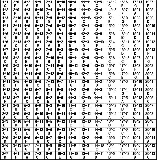
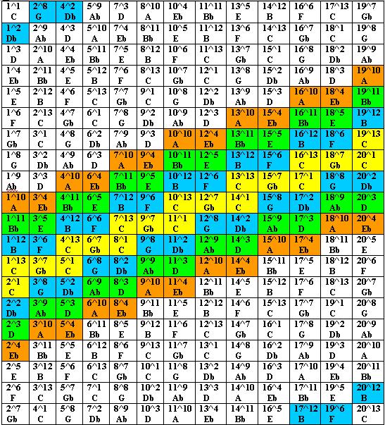